Document Updated last:
sysSt <- Sys.time()
sysSt
## [1] "2017-08-15 23:03:38 EDT"
This paper illustrates an ensemble model approach for the Ames House Price data. An ensemble model combines multiple models in an effort to increase the predictive accuracy. This specific ensemble approach illustrates the model stacking method.
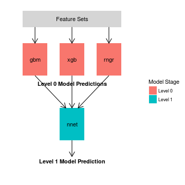
The diagram below shows the high-level model stacking architecture, which is composed of two stages. The top-level stage, called Level 0, is composed of three modeling algorithms:
- Gradient Boosting (gbm)
- Extreme Gradient Boosting (xgb)
- Random Forest (rngr)
The second stage, Level 1, is composed of a single Neural Network (nnet) model. The predictions from Level 1 are used to create the final data set.
Feature Sets in the diagram represents one or more sets of attributes created for the Level 0 models.

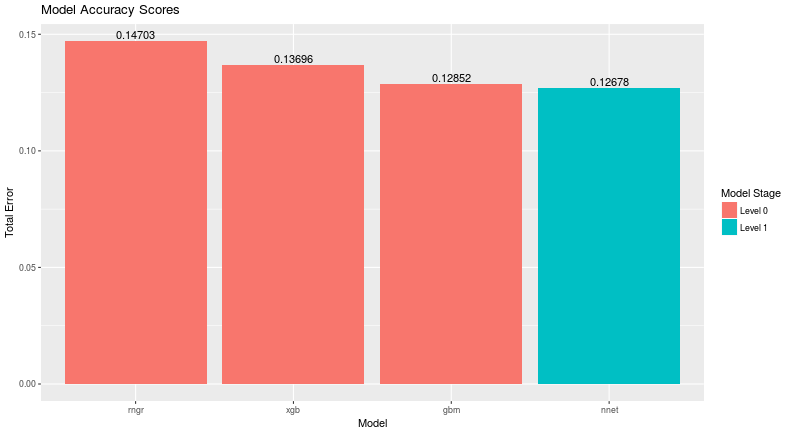
The following chart shows the model performance of the individual Level 0 models versus the overall stacked model.
##   Model PLB_Score   Level
## 1   gbm   0.12852 Level 0
## 2   xgb   0.13696 Level 0
## 3  rngr   0.14703 Level 0
## 4  nnet   0.12678 Level 1
The percent reduction for the Level 1 model compared to the best performing Level 0 model:
## [1] 1.353875

From the above chart we see that the Level 1 model is a 1.35% improvement over the best performing Level 0 model.
To fit within the constraints of an intuitive ensemble model approach, a simple stacked model was designed. A performance gain for Level 1 predictive power supports the simple design efficacy. The wisdom of Occum’s Razor, i.e. parsimony, cannot be overstated when designing models. A simple model design supports efficient model optimization. The specific simplications are
- Limit Level 0 to three models
- Limit Level 1 to one model
Improvements in stacked model performance can be accomplished by
- Adding models to Level 0 and Level 1 using different algorithms
- Tuning model Hyper-parameters
- Adding feature sets by feature engineering
- Adding levels in the model structure
The remainder of this paper demonstrates the model stacking training pipeline. First we show an approach for creating model feature sets. Next we demonstrate an approach for training Level 0 models.
Then we end with creating features for the Level 1 model and creating the final data set.
Data Preparation
Retrieve Data
Initial Data Profile
Feature selection is based on a wrapper algorithm for feature importance analysis. The full set of variables includes SalePrice (y-variable) and 79 predictors (x-variables). Most variables have informative descriptive names.
##  [1] "MSSubClass"    "MSZoning"      "LotArea"       "LotShape"
##  [5] "LandContour"   "Neighborhood"  "BldgType"      "HouseStyle"
##  [9] "OverallQual"   "OverallCond"   "YearBuilt"     "YearRemodAdd"
## [13] "Exterior1st"   "Exterior2nd"   "MasVnrArea"    "ExterQual"
## [17] "Foundation"    "BsmtQual"      "BsmtCond"      "BsmtFinType1"
## [21] "BsmtFinSF1"    "BsmtFinType2"  "BsmtUnfSF"     "TotalBsmtSF"
## [25] "HeatingQC"     "CentralAir"    "X1stFlrSF"     "X2ndFlrSF"
## [29] "GrLivArea"     "BsmtFullBath"  "FullBath"      "HalfBath"
## [33] "BedroomAbvGr"  "KitchenAbvGr"  "KitchenQual"   "TotRmsAbvGrd"
## [37] "Functional"    "Fireplaces"    "FireplaceQu"   "GarageType"
## [41] "GarageYrBlt"   "GarageFinish"  "GarageCars"    "GarageArea"
## [45] "GarageQual"    "GarageCond"    "PavedDrive"    "WoodDeckSF"
## [49] "OpenPorchSF"   "Fence"         "Alley"         "LandSlope"
## [53] "Condition1"    "RoofStyle"     "MasVnrType"    "BsmtExposure"
## [57] "Electrical"    "EnclosedPorch" "SaleCondition" "LotFrontage"
## [61] "Street"        "Utilities"     "LotConfig"     "Condition2"
## [65] "RoofMatl"      "ExterCond"     "BsmtFinSF2"    "Heating"
## [69] "LowQualFinSF"  "BsmtHalfBath"  "X3SsnPorch"    "ScreenPorch"
## [73] "PoolArea"      "PoolQC"        "MiscFeature"   "MiscVal"
## [77] "MoSold"        "YrSold"        "SaleType"
Create Level 0 Model Feature Sets
Machine learning algorithms perform better when uninformative predictors are removed. For this work, two feature sets were created. Both of these sets included Boruta (wrapper algorithm) confirmed and tentative attributes.
Each feature set is created by a specific user-defined R function. These functions
convert the raw training data into a feature set.
No extensive feature engineering was performed. Missing values are handled as
follows:
- Numeric: set to -1
- Character: set to “*MISSING*”
Character attributes are converted to R factor variables.
Level 0 Model Training
Helper Function For Training
Data is split up into train and test, using an 80/20 split.
gbm Model
Generalized Boosted Regression Model
Score: 0.12852
## [1] 0.1309466
## Average CV rmse: 0.1304117
xgboost Model
Extreme Gradient Boosting
Score: 0.13696
## [1] 11.53097
## Average CV rmse: 11.53097
ranger Model
Random Forest
Score: 0.14703
## [1] 0.138126
## Average CV rmse: 0.1369463
Level 1 Model Training
Create predictions For Level 1 Model
Neural Net Model
Score: 0.12678
## Average CV rmse: 0.1270413
References
Additional Resources
For additional information on model stacking see these references:
- MLWave: Kaggle Ensembling Guide
- Kaggle Forum Posting: Stacking
- Winning Data Science Competitions: Jeong-Yoon Lee This talk is about 90 minutes long. The sections relevant to model stacking are discussed in
these segments (h:mm:ss to h:mm:ss): 1:05:25 to 1:12:15 and 1:21:30 to 1:27:00.
Document Utilities
## [1] "2017-08-15 23:01:13 EDT"
## Time difference of 1.164407 mins
## [1] "/media/disc/Megasync/R_wordpress/ensemble_stacked_model"
## [1] "cache"                       "ensemble_stacked_wp_cache"
## [3] "ensemble_stacked_wp_files"   "ensemble_stacked_wp.html"
## [5] "ensemble_stacked_wp.nb.html" "ensemble_stacked_wp.Rmd"
## [7] "figure"
## R version 3.3.3 (2017-03-06)
## Platform: x86_64-pc-linux-gnu (64-bit)
## Running under: Ubuntu 16.04.2 LTS
##
## locale:
##  [1] LC_CTYPE=en_US.UTF-8       LC_NUMERIC=C
##  [3] LC_TIME=en_US.UTF-8        LC_COLLATE=en_US.UTF-8
##  [5] LC_MONETARY=en_US.UTF-8    LC_MESSAGES=en_US.UTF-8
##  [7] LC_PAPER=en_US.UTF-8       LC_NAME=C
##  [9] LC_ADDRESS=C               LC_TELEPHONE=C
## [11] LC_MEASUREMENT=en_US.UTF-8 LC_IDENTIFICATION=C
##
## attached base packages:
## [1] parallel  splines   stats     graphics  grDevices utils     datasets
## [8] methods   base
##
## other attached packages:
##  [1] e1071_1.6-8      gbm_2.1.3        survival_2.41-3  bindrcpp_0.1
##  [5] Metrics_0.1.2    nnet_7.3-12      ranger_0.7.0     xgboost_0.6-4
##  [9] dplyr_0.5.0.9004 plyr_1.8.4       caret_6.0-76     ggplot2_2.2.1
## [13] lattice_0.20-35  markdown_0.7.7   knitr_1.15.1     RWordPress_0.2-3
##
## loaded via a namespace (and not attached):
##  [1] reshape2_1.4.2     colorspace_1.3-2   stats4_3.3.3
##  [4] mgcv_1.8-17        XML_3.98-1.9       rlang_0.0.0.9018
##  [7] ModelMetrics_1.1.0 nloptr_1.0.4       glue_1.0.0
## [10] foreach_1.4.3      bindr_0.1          stringr_1.2.0
## [13] MatrixModels_0.4-1 munsell_0.4.3      gtable_0.2.0
## [16] codetools_0.2-15   evaluate_0.10      labeling_0.3
## [19] SparseM_1.76       class_7.3-14       quantreg_5.29
## [22] pbkrtest_0.4-7     XMLRPC_0.3-0       highr_0.6
## [25] Rcpp_0.12.10       scales_0.4.1       lme4_1.1-12
## [28] digest_0.6.12      stringi_1.1.3      grid_3.3.3
## [31] tools_3.3.3        bitops_1.0-6       magrittr_1.5
## [34] lazyeval_0.2.0     RCurl_1.95-4.8     tibble_1.3.0
## [37] car_2.1-4          MASS_7.3-45        Matrix_1.2-8
## [40] data.table_1.10.4  assertthat_0.2.0   minqa_1.2.4
## [43] iterators_1.0.8    R6_2.2.0           compiler_3.3.3
## [46] nlme_3.1-131